Ammm:Free energy simulations

Free Energy Calculations

• Equilibrium Methods (FEP, TI)
• Nonequilibrium Methods

Density of States

• $\Omega$ = density of states
• $1/h^{3N}$ = factor of proportionality (necessary to retrieve correct correspondence with high-temperature quantum-mechanical prediction)

• Calculations

• In canonical ensemble, $A=-\beta \ln {Q(N,V,T)}$

Ergodicity

• The ergodic hypothesis allows generating trajectories (i.e. MD, MC) to sample from phase-space to compute ensemble averages.
• The ensemble average of the property $f$ of a system is:

$\left\langle f\right\rangle =\int fP(\mathbf {x} ,\mathbf {p} _{x})d\mathbf {x} d\mathbf {p} _{x}$

• The ergodic hypothesis states that

$\left\langle f\right\rangle =\lim _{T\rightarrow \infty }{\frac {1}{T}}\int _{0}^{T}f[\mathbf {q} (t),\mathbf {p} (t)]dt$ for any $\mathbf {q_{0}} =\mathbf {q} (0),\mathbf {p_{0}} =\mathbf {p} (0)$

• Quasi-nonergodic - a system that does not explore phase space over time.
  • high energy barriers separating volumes of phase space
  • volume in phase space diffuses very slowly
• Proof of Quasi-ergodic hypothesis
• Proof of ergodic theorem

Free Energy Perturbation

Perturbation Formalism

• We want to calculate the free energy difference between state 0 and state 1 of Hamiltonians ${\mathcal {H}}_{0}(\mathbf {x} ,\mathbf {p} _{x})$ and ${\mathcal {H}}_{1}(\mathbf {x} ,\mathbf {p} _{x})$

• The difference in Helmholtz free energy between is $\Delta A=-{\frac {1}{\beta }}\ln {\frac {Q_{1}}{Q_{0}}}$ where $\beta =(k_{B}T)^{-1}$

• $Q_{0}$ and $Q_{1}$ are their corresponding partition functions $Q={\frac {1}{h^{3N}N!}}\iint \exp[-\beta {\mathcal {H}}]d\mathbf {x} d\mathbf {p} _{x}$

• $\Delta A=-{\frac {1}{\beta }}\ln {\frac {\iint \exp[-\beta {\mathcal {H}}_{1}(\mathbf {x} ,\mathbf {p} _{x})]d\mathbf {x} d\mathbf {p} _{x}}{\iint \exp[-\beta {\mathcal {H}}_{0}(\mathbf {x} ,\mathbf {p} _{x})]d\mathbf {x} d\mathbf {p} _{x}}}$

• $\Delta A=-{\frac {1}{\beta }}\ln {\frac {\iint \exp[-\beta \Delta {\mathcal {H}}(\mathbf {x} ,\mathbf {p} _{x})]\exp[-\beta {\mathcal {H}}_{0}(\mathbf {x} ,\mathbf {p} _{x})]d\mathbf {x} d\mathbf {p} _{x}}{\iint \exp[-\beta {\mathcal {H_{0}}}]d\mathbf {x} d\mathbf {p} _{x}}}$

• $\Delta A=-{\frac {1}{\beta }}\ln \iint \exp[-\beta \Delta {\mathcal {H}}(\mathbf {x} ,\mathbf {p} _{x})]P_{0}(\mathbf {x} ,\mathbf {p} _{x})d\mathbf {x} d\mathbf {p} _{x}$
  • since $P_{0}(\mathbf {x} ,\mathbf {p} _{x})={\frac {\exp[-\beta \Delta {\mathcal {H}}_{0}(\mathbf {x} ,\mathbf {p} _{x})]}{\iint \exp[-\beta {\mathcal {H}}_{0}(\mathbf {x} ,\mathbf {p} _{x})]d\mathbf {x} d\mathbf {p} _{x}}}$

• Finally, $\Delta A=-{\frac {1}{\beta }}\ln \left\langle \exp[-\beta \Delta {\mathcal {H}}(\mathbf {x} ,\mathbf {p} _{x})]\right\rangle _{0}$

• For systems of with the same masses, $\Delta A=-{\frac {1}{\beta }}\ln \left\langle \exp[-\beta \Delta U]\right\rangle _{0}$

• We can also swap states 0 and 1 and use $\Delta A=-{\frac {1}{\beta }}\ln \left\langle \exp[-\beta \Delta U]\right\rangle _{1}$
  • Although forward and backward calculations are formally equilvalent, they may have different convergence properties

• Forward and backward calculations can be combined (BAR).

Stratification

• P($\Omega$) is a probability distribution over the domain $\Omega$
• Partition $\Omega$ in to disjoint regions $\Omega _{i}\subset \Omega$ so that $\bigcup _{i\epsilon I}\Omega _{i}=\Omega$
• Example
  • Consider a transformation of state 0 to state 1 described by parameter $\lambda$
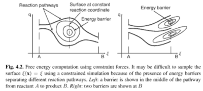
  • Suppose states 0 and 1 are separated by a high-energy barrier
  • Partition $\lambda$ in to a number of smaller intervals
  • P($\lambda$) can be recovered with great savings in computer time
• Decreases variance of ensemble average
• Provides solution for quasi-nonergodic systems

Importance sampling

• Sample regions in phase space that are important for estimating quantity of interest more frequently
• Results of the simulation need to be weighted to ensure that estimator is unbiased
• Example
  • Transformation from state 0 to state 1 along $\lambda$
  • Define P($\lambda$) to be the true distribution
  • Let $P'(\lambda )=P(\lambda )\exp[\beta \eta (\lambda )]$ where $\eta (\lambda )$ is the weighting factor
  • Then $\Delta A=-\beta ^{-1}\ln {\frac {P(\lambda _{1})}{P(\lambda _{0})}}=-\beta ^{-1}\ln {\frac {P'(\lambda _{1})}{P'(\lambda _{0})}}+\eta (\lambda _{1})-\eta (\lambda _{0})$

Order Parameter

• Coupling parameters, $\lambda$, that are used to describe transformations from the reference system to the target one.
• Reaction coordinate/path - an order parameters that corresponds to the path along which the transformation takes place in nature
• Examples
  • Simple/coupled torsional degrees of freedom
  • End-to-end reaction coordinate (for protein folding)
  • Mutagenesis of atoms (relative free energy)
  • Distance separating chemical species (PMF)
  • Annihilation of nonbonded interactions (solvation)
• Choice of $\lambda$ significantly affects efficiency, accuracy of calculations
  • Smooth energy landscapes require less intermediate states than rough ones

Topology

• Single Topology paradigm - a common topology is used for initial and final states
  • Missing atoms are treated as vanishing particles by setting nonbonded parameters to 0.
  • Bonded terms
    • If chemical bonds are not strongly deformed between initial and target states, bonded terms are often not considered
    • However, FEP and TI can simulations can be used as well.
  • Examples of systems that can use single topology

• Dual Topology paradigm -
  • States 0 and 1 contain different topologies
  • Atoms not common to 0 and 1 never interact during the simulation.
  • Bonded parameters are not perturbed

• • 

Thermodynamic Cycle

• Hydration free energy of a small solute
  • $\Delta A_{hydration}=\Delta A_{0}-\Delta A_{1}$

• Binding free energy of ligand to protein
  • $\Delta A_{binding}=\Delta A_{0}-\Delta A_{1}$

• Relative binding free energy of ligand to protein
  • $\Delta \Delta A_{AB}=\Delta A_{bind\!-\!B}-\Delta A_{bind\!-\!A}=\Delta A_{1}-\Delta A_{0}$

Application of FEP

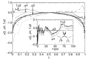
• Enthalpy and entropy can be computed based on their thermodynamic relationship using finite difference.
• $\Delta S=\partial \Delta A/\partial T$
• $\Delta U=\partial \beta \Delta A/\partial \beta$
• 

Thermodynamic Integration

• If $\xi$ is a reaction coordinate, the free energy is $A(\xi )=-k_{B}T\ln P(\xi )$
• For a sufficiently smooth function, free energy difference can be written as $A(\xi _{1})-A(\xi _{0})=\int _{\xi _{0}}^{\xi _{1}}dA/d\xi \,d\xi$ where ${\frac {dA}{d\xi }}=\left\langle {\frac {\partial {\mathcal {H}}}{\partial \xi }}\right\rangle _{\xi }$
• Order parameters can be torsion angle, bond lengths/angles between atoms or groups of atoms, hydration number, gyration radius

Constrained Simulations

• The Hamiltonian is supplemented by a Langrange multiplier

${\mathcal {H}}^{\lambda }\equiv {\mathcal {H}}+\lambda (\xi -\xi (\mathbf {x} ))=K+U+\lambda (\xi -\xi (\mathbf {x} ))$

• Since $\xi (\mathbf {x} )$ is constant, ${\ddot {\xi }}=0$ we have

$\lambda =Z_{\xi }^{-1}\left(\sum _{i}{\frac {1}{m_{i}}}{\frac {\partial \xi }{\partial x_{i}}}{\frac {\partial U}{\partial x_{i}}}-{\dot {\mathbf {x} }}^{t}\cdot \mathbf {H} \cdot {\dot {\mathbf {x} }}\right)$ where $Z_{\xi }=\sum _{i}{\frac {1}{m_{i}}}\left({\frac {\partial \xi }{\partial x_{i}}}\right)^{2}$ and $\mathbf {H} _{ij}={\frac {\partial ^{2}\xi }{\partial x_{i}\partial x_{j}}}$ is the hessian of $\xi$

• $A(\xi )=\int \langle \lambda \rangle _{\xi ,{\dot {\xi }}}d\xi -k_{b}T\ln \langle Z_{\xi }^{-1/2}\rangle$

Adaptive Biasing Force Method

• 
• ${\frac {dA}{d\xi }}=-\left\langle {\frac {d}{dt}}\left(m_{\xi }{\frac {d\xi }{dt}}\right)\right\rangle$ where $m_{\xi }=Z_{\xi }^{-1}$
• Using velocity verlet integrator where:
  • $v(t+dt/2)=v(t-dt/2)+dt\;a(t)$
  • $x(t+dt/2)=x(t)+dt/2\;v(t+dt/2)$
• ${\frac {d}{dt}}\left(m_{\xi }{\frac {d\xi }{dt}}\right)={\frac {1}{2}}\left({\frac {p_{\xi }^{+}(t+dt)-p_{\xi }^{+}(t)}{dt}}+{\frac {p_{\xi }^{-}(t+dt)-p_{\xi }^{-}(t)}{dt}}\right)$

where $p_{\xi }^{+}(t)\equiv m_{\xi }(t)grad(\xi (t))\cdot \left[v(t+dt/2)-{\frac {dt}{6}}a(t+dt)\right]$ and $p_{\xi }^{-}(t)\equiv m_{\xi }(t)grad(\xi (t))\cdot \left[v(t-dt/2)-{\frac {dt}{6}}a(t-dt)\right]$

• Ramping function is used to prevent nonequilibrium effects and systematic bias in the beginning of the simulation.

$R(n)={\begin{cases}n/N_{0}&{\textrm {if}}\;n\leq N_{0}\\1&{\textrm {if}}\;n>N_{0}\\{\textrm {with}}\;N_{0}\cong 100\end{cases}}$

Examples

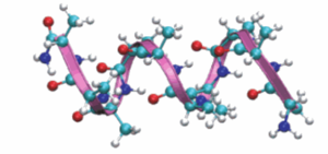
Deca-L-alanine

• ABF was used to probe the reversible unfolding of deca-L-alanine in vacuo
• The reaction coordinate is the distance separating first and last alpha carbon from 12-32 Angstrom
  • 5ns MD trajectory
• 
• Minimum at around 14 Angstrom
• 
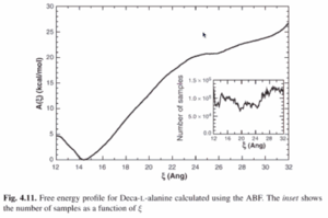
• Free energy profile essentially identical to a reversible, 20-ns steered MD simulation
• Park et al.

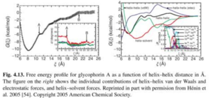
Glycophorin A

• ABF was used to model the helix-helix association of Glycophorin A
• 
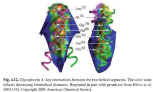
• Difficulty of this simulation is that once the two helices are close to each other, it is very difficult to slide one with respect to the other or change relative orientation due to steric clashes.
• Constrained sampling would keep positions in local minimum in phase-space.
•

References

- ↑ Frenkel, D.; Smit, B., Understanding molecular simulation: from algorithms to applications. Academic: San Diego, Calif. London, 2002.
- ↑ Chipot, C.; Pohorille, A., Free Energy Calculations - Theory and Applications in Chemistry and Biology. Springer-Verlag: Berlin Heidelberg, 2007; Vol. 86.
- ↑ http://www.ncbi.nlm.nih.gov/pmc/articles/PMC1076162
- ↑ http://www.ncbi.nlm.nih.gov/pmc/articles/PMC1076138
- ↑ Jiao, D.; Zhang, J.; Duke, R. E.; Li, G.; Schnieders, M. J.; Ren, R. J. Comput. Chem. 2009, 30, 1701– 1711.
- ↑ http://www.ks.uiuc.edu/Research/namd/2.6/ug/node36.html#fig:dual_top
- ↑ E. Darve and A. Pohorille, J. Chem. Phys. 115, 9169 (2001).
- ↑ Park, S.; Khalili-Araghi, F.; Tajkhorshid, E.; Schulten, K., Free energy ccalculation from steered molecular dynamics simulatiosn using Jarzynski's equality, J. Chem. Phys. 2003, 119, 3559-3566.