Ammm:Umbrella sampling and WHAM

Reaction Coordinate

• A reaction coordinate is an abstract one-dimensional coordinate which represents progress along a reaction pathway.
  • Real coordinate system: bond length, bond angle, torsion
  • Non geometric parameters: bond order, Hydrogen bonds, RMSD
• Reaction coordinates are often plotted against free energy to demonstrate in some schematic form the potential energy profile associated to the reaction.

Umbrella Sampling (US)

Umbrella sampling is a method in computational physics and chemistry, which can enhance the sampling of different systems when it is hard to realize ergodicity due to the energy landscape. It involves the importance sampling in statistical mechanics and was first recommended by Torrie and Valleau in 1977.In many cases, the configuration space may have multiple high-energy barriers which are hard to conquer in the limited simulation time with common molecular dynamics (MD). Therefore, it is of high probability that the trajectory is trapped in the local minimum (local state) and leaves other inaccessible important states unsampled. In order to remove the impact of the energy barriers (activation case), the researchers can chosose the umbrella sampling (US) to bridge the gap between different configuration states by adding an extra bias potential. This bias potential should cancel out the influence of these energy barriers so that the energy landscape will become more smooth, making it easier to reach other states.

Why do we need biased potential?

Features of method

• Pre-determined collective variables are required to describe the configuration space related to reaction.
• The target of this method is to handle activation problems in sampling, where high energy barriers can be smoothened by adding extra bias potential. (Convert activation into diffusion)
• The extra bias potential causes the loss of temporal properties.
• This method supports parallel MD simulations with different bias potentials at the same time so that computational cost is reduced.
• This method demands post-processing to remove the effects of bias potential.

Weighted ensemble

The original ensemble can be modified by using a weight function. The weight function should be positive here.

$<exp(-\beta \Delta U)>_{0}={\frac {\int \,exp(-\beta \Delta U)exp(-\beta \Delta U_{0})dx}{\int \,exp(-\beta \Delta U_{0})dx}}$

$<exp(-\beta \Delta U)>_{0}={\frac {\int \,exp(-\beta \Delta U)ww^{-1}exp(-\beta \Delta U_{0})dx}{\int \,exp(-\beta \Delta U_{0})ww^{-1}dx}}={\frac {<w^{-1}exp(-\beta \Delta U)>_{w}}{<w^{-1}>_{w}}}$

In the equation above, the $<...>_{w}$ denotes the weighted ensemble average and the probability distribution function can be shown as:

$\rho _{w}(x)={\frac {wexp(-\beta \Delta U_{0})}{\int \,wexp(-\beta \Delta U_{0})dx}}$

To reflect the connection between bias potential and the weight function, we can represent the weight function as an exponential form: $w=exp(-\beta V)$, where $V$ means the bias potential.

$<exp(-\beta \Delta U)>_{0}={\frac {<exp(\beta V)exp(-\beta \Delta U)>_{w}}{<exp(\beta V)>_{w}}}$

Free energy calculation

After defining a collective variable (CV) $\xi$, we can calculate the free energy at any point along the direction of CV by using the probability distribution function. (The reference point is chosen at $\xi _{0}$)

$\Delta A(\xi )=-k_{B}Tln{\frac {\rho _{0}(\xi )}{\rho _{0}(\xi _{0})}}$

When the bias potential is added, the free energy change under the weighted ensemble can be given by:

$\Delta A_{w}(\xi )=-k_{B}Tln{\frac {\rho _{w}(\xi )}{\rho _{w}(\xi _{0})}}$

In this case, the original free energy change should be recovered by combining these two equations above: (the denominators have been offset in the ratio)

$\Delta A(\xi )=-k_{B}Tln{\frac {\rho _{w}(\xi )w(\xi _{0})}{\rho _{w}(\xi _{0})w(\xi )}}$

$\Delta A(\xi )=\Delta A_{w}(\xi )+k_{B}T(lnw(\xi )-lnw(\xi _{0}))=\Delta A_{w}(\xi )-[V(\xi )-V(\xi _{0})]$

The best bias potential can help remove all the possible barriers on the energy landscape, which means the free energy change under this bias potential should be 0 everywhere. So, it is obvious to know that the best bias potential must counterbalance the true free energy.

$V(\xi )-V(\xi _{0})=-\Delta A(\xi )$

Challenges of Umbrella Sampling

• Pick up the best bias potential along the CVs to realize the sufficiently flat energy landscape
• Ensure complete scanning of all the configuration space along the CVs under bias potential
• Perform discretization of the probability distribution along CVs

WHAM

Historty

• Initially developed in 1989 by Ferrenberg and Swenden: Ferrenberg-Swenden reweighting
• Generalized by Kumar et al.: Weighted Histogram Analysis Method

Basic Idea

The Weighted Histogram Analysis Method (WHAM) is a practical technique for the calculation of potentials of mean force (PMFs) from a group of umbrella sampling simulations. It can be applied to analyze the energy data based on not only real collective variables (have relations to the atom coordinates) but also virtual variables (temperature or interactions in the system). This technique can give out a systematic way to improve the choice of the bias potential from a set of different bias potentials so that it yields uniform sampling along the collective variables. Meanwhile, the multiple simulations can start from different points along collective variables, then the full sampling can be realized. Also, the underlying theory of this method provides us with a practical way to do histogram analysis and calculate free energy under discretized language.

Discretization of configuration space along collective variable

Assume we have run $R$ simulations at the same time, with each using a different or same bias potential and temperature. ${\displaystyle }$

$U_{k}=U_{0}+V_{k}(\xi ),k=1,...,R$

The whole configuration space can be divided into $L$ bins. The middle bins share the same width $d$ while the beginning and end bins have the width $d/2$. After the division, the configuration space becomes a histogram graph, and the energy value for each bin $i$ in simulation $k$ should be given by the following equation: (energy for middle bins is set to be the value of the middle point of this bin, while the energy of the beginning bin is set to be the value at the starting point and the energy of the end bin is set to be the value at the endpoint)

$V_{k,i}={\begin{cases}V_{k}(\xi _{i}),&(i=1,L+1)\\V_{k}({\frac {\xi _{i}+\xi _{i+1}}{2}}),&(i=2,...,L)\end{cases}}$

Then, the bias potential energy of the simulation $k$ along collective variable can be expressed in discretized language:

$V_{k}(\xi )=\sum _{i=1}^{L}V_{k,i}\chi _{[\xi _{i},\xi _{i+1}]}(\xi )$

$\chi _{[\xi _{i},\xi _{i+1}]}$ is characteristic function: if $\xi$ is in the range $[\xi _{i},\xi _{i+1}]$ then it takes value $1$, otherwise it is $0$.

From the operation of dividing the whole configuration space into discrete bins, it is obvious that more bins indicate higher resolution, but more snapshots from the simulations are required. To make the expression more clear, we directly use $V_{k,i}(\xi )$ to denote the function $V_{k,i}\chi _{[\xi _{i},\xi _{i+1}]}(\xi )$ in the following.

State density & probability distribution function

The most important property in WHAM is state density (or energy state density) $\Omega$. In an NVT ensemble, the generalized state density can be shown as:

$\Omega (N,V,U)={\frac {1}{h^{3N}N!}}\iint \limits _{V^{3N}}\delta (H(\mathbf {q} ,\mathbf {p} )-U)\,d\mathbf {q} \,d\mathbf {p}$

then $\Omega (N,V,U)dU$ represents the volume of microstates in $[U-dU/2,U+dU/2]$. The partition function can be illustrated by using state density:

$Q(N,V,T)=\int \limits exp(-\beta U)\Omega (N,V,U)\,dU$

$Q(N,V,T)={\frac {1}{h^{3N}N!}}\iint \limits _{V^{3N}}exp(-\beta U(\mathbf {q} ,\mathbf {p} ))\,d\mathbf {q} \,d\mathbf {p} ={\frac {1}{\Lambda ^{3N}N!}}\int \limits exp(-\beta U(\mathbf {q} ))\,d\mathbf {q} ={\frac {1}{\Lambda ^{3N}N!}}Z(N,V,T)$

$Z(N,V,T)$ is the configurational integral. From these equations above, the probability distribution function can be expressed as:

$\rho (U;N,V,T)={\frac {exp(-\beta U)\Omega (N,V,U)}{Z(N,V,T)}}$

In WHAM, the probability and state density can be calculated by using statistical data: $N_{k}(\xi )$ is the number of counts at $\xi$ in simulation $k$, $n_{k}$ is the total number of snapshots in simulation $k$.

$\rho _{k}(U(\xi ),T_{k})={\frac {N_{k}}{n_{k}}}={\frac {exp(-\beta _{k}U)\Omega _{k}(U)}{Z_{k}}}$

$\Omega _{k}(U)=a_{k}{\frac {N_{k}}{n_{k}}}exp(-\beta _{k}U)$

$a_{k}$ denotes the proportionality constant unique for k-th simulation (related to configurational integral), which can be modified further to make the following equations more pretty: $a_{k}=exp(-\beta _{k}f_{k})$.

Derivation of WHAM

When bias potential is shown explicitly, the state density becomes:

$\Omega _{k}(\xi )={\frac {N_{k}}{n_{k}}}exp(\beta _{k}U_{0}(\xi )+\sum _{i=1}^{L}\beta _{k}V_{k,i}(\xi )-\beta _{k}f_{k})$

Because the original energy distribution is the same for all the simulations and will be reduced in the following deduction, then we can remove that in state density.

$\Omega _{k}(\xi )={\frac {N_{k}}{n_{k}}}exp(\sum _{i=1}^{L}\beta _{k}V_{k,i}(\xi )-\beta _{k}f_{k})$

The state density with the best bias potential can be given by a linear combination of state density functions from all $R$ simulations, with each one being assigned a weight $\omega _{k}$. The sum of all the weights should be $1$.

$\Omega (\xi )=\sum _{k=1}^{R}\omega _{k}\Omega _{k},\sum _{k=1}^{R}\omega _{k}=1$

To get the best state density, we need to minimize the mean square deviation (MSD) $\delta ^{2}\Omega$

$\delta ^{2}\Omega =\sum _{k=1}^{R}\omega _{k}^{2}\delta ^{2}\Omega _{k}$

$\delta ^{2}\Omega _{k}={\frac {1}{n_{k}^{2}}}exp(\sum _{i=1}^{L}\beta _{k}V_{k,i}-\beta _{k}f_{k})\delta ^{2}N_{k}$

The MSD of $N_{k}$ can be given by multiplication of a correlation factor and its average: (the correlation factor is roughly equal if the division and running time are the same for all simulations, so it can be canceled)

$\delta ^{2}N_{k}(\xi )=g_{k}{\bar {N_{k}}}(\xi )$

An estimate can be made to obtain the average ${\bar {N}}_{k}$:

$\Omega (\xi )={\frac {{\bar {N_{k}}}(\xi )exp(\sum _{i=1}^{L}\beta _{k}V_{k,i}(\xi )-\beta _{k}f_{k})}{n_{k}}}$

which can be compared with $\Omega _{k}(\xi )={\frac {N_{k}(\xi )exp(\sum _{i=1}^{L}\beta _{k}V_{k,i}(\xi )-\beta _{k}f_{k})}{n_{k}}}$.

Then: ${\bar {N_{k}}}(\xi )=n_{k}\Omega (\xi )exp(-\sum _{i=1}^{L}\beta _{k}V_{k,i}(\xi )+\beta _{k}f_{k})$.

The minimization can be finished by using the method of Lagrangian multipliers:

${\frac {\partial (\delta ^{2}\Omega )}{\partial \omega _{k}}}={\frac {\partial }{\partial \omega _{k}}}(\delta ^{2}\Omega +\lambda (\sum _{i}\omega _{i}-1))$

$2\omega _{k}\delta ^{2}\Omega _{k}+\lambda =0(k=1,...,R)$

$\omega _{1}\delta ^{2}\Omega _{1}=\omega _{2}\delta ^{2}\Omega _{2}=...=\omega _{R}\delta ^{2}\Omega _{R}=C$

Because $\sum {i}\omega _{i}=1$, then $C={\frac {1}{\sum _{k}{\frac {1}{\delta ^{2}\Omega _{k}}}}}$.

$\omega _{k}={\frac {\delta ^{2}\Omega _{k}}{\sum _{k}{\frac {1}{\delta ^{2}\Omega _{k}}}}}={\frac {g_{k}^{-1}n_{k}exp(-\sum _{i=1}^{L}\beta _{k}V_{k,i}(\xi )+\beta _{k}f_{k})}{\sum _{m=1}^{R}g_{m}^{-1}n_{m}exp(-\sum _{i=1}^{L}\beta _{m}V_{m,i}(\xi )+\beta _{m}f_{m})}}$.

Then:

$\Omega (\xi )=\sum _{k=1}^{R}\omega _{k}\Omega _{k}(\xi )={\frac {\sum _{k=1}^{R}g_{k}^{-1}N_{k}(\xi )}{\sum _{m=1}^{R}g_{m}^{-1}n_{m}exp(-\sum _{i=1}^{L}\beta _{m}V_{m,i}(\xi )+\beta _{m}f_{m})}}$

In bin $i$:

$\Omega _{,i}={\frac {\sum _{k=1}^{R}g_{k}^{-1}N_{k,i}}{\sum _{m=1}^{R}g_{m}^{-1}n_{m}exp(-\sum _{i=1}^{L}\beta _{m}V_{m,i}+\beta _{m}f_{m})}}$

The un-normalized density at bin $i$ in simulation $K$ can be given by:

${\tilde {\rho }}_{K,i}={\frac {exp(-\beta _{K}V_{K,i})\sum _{k=1}^{R}g_{k}^{-1}N_{k,i}}{\sum _{m=1}^{R}g_{m}^{-1}n_{m}exp(-\sum _{i=1}^{L}\beta _{m}V_{m,i}+\beta _{m}f_{m})}}\ \ (*)$

Because $f_{K}$ is related to configurational integral:

$exp(-\beta _{K}f_{K})=\sum _{i=1}^{L}{\tilde {\rho }}_{K,i}\ \ (**)$

The most common case is that all the temperatures are the same, and the correlation factors are cancelled out. Then the equations $(*)$ and $(**)$ can be simplified into:

${\tilde {\rho }}_{K,i}={\frac {exp(-\beta V_{K,i})\sum _{k=1}^{R}N_{k,i}}{\sum _{m=1}^{R}n_{m}exp(-\sum _{i=1}^{L}\beta V_{m,i}+\beta f_{m})}}\ \ (*)$

$exp(-\beta f_{K})=\sum _{i=1}^{L}{\tilde {\rho }}_{K,i}\ \ (**)$

Self-consistent algorithm

In equations $(*)$ and $(**)$, the unknown values are $f_{K}$ and ${\tilde {\rho }}_{K,i}$. We can work out their values by using the self-consistent method.

At first, we can assume $f_{K}=0(K=1,...,R)$ and put them into Equation $(*)$ to obtain ${\tilde {\rho }}_{K,i}(K=1,..,R;i=1,...,L)$.

Next step: Put all ${\tilde {\rho }}_{K,i}$ into Equation $(**)$ to get the values of $f_{K}$.

Repeat the two steps above until the deviations of all these values are smaller than pre-set tolerance. The true free energy change between any two bins in simulation $K$ without bias potential can be calculated by:

$\Delta A_{K,j\to i}=-\beta _{K}^{-1}ln({\frac {\rho _{K,i}}{\rho _{K,j}}})$

Procedure of umbrella sampling

• Define collective variables appropriate to describe the reaction space
• Divide the whole reaction space into bins with proper resolution
• Generate different configurations at each bin by using steered MD (or directly do pulling during different simulations)
• Set bias potential for each configuration (commonly used: harmonic restrain)
• Run multiple MDs with different bias potentials and record the trajectories & energy
• Put data into the WHAM processing program (use the module from Gromacs, …)

Examples

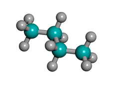
Butane

• Protocol
  • 18 independent simulations
    • 500ps
    • Restraint spring constant = 0.02 kcal/mol-deg
  • WHAM
    • 90 bins (40/bin)
    • Enforced periodcity

• Histograms from Individual Trajectories

• Histograms of Combined Trajectories

• Butane PMF

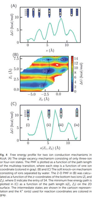
Ion Channel

Tutorial of US & WHAM

The Gromacs provides us with a good tutorial to show the way to perform Umbrella Sampling & WHAM post-processing: http://www.mdtutorials.com/gmx/umbrella/

References

- ↑ Torrie, G. M.; Valleau, J. P. (1977). "Nonphysical sampling distributions in Monte Carlo free-energy estimation: Umbrella sampling". Journal of Computational Physics. 23 (2): 187–199. doi:10.1016/0021-9991(77)90121-8
- ↑ Ferrenberg; Swenden, Optimized Monte Carlo data Analysis, Phys.Rev.Lett. 1989, 63, 1195-1198
- ↑ Kumar S, Bouzida D, Swendsen RH, Kollmann PA, Rosenberg JM: The weighted histogramfckLRanalysis method for free-energy calculations on biomolecules. I. The method. J Comp ChemfckLR1992, 13: 1011-1021.
- ↑ Roux B: Extension to the weighted histogram analysis method: combining umbrella sampling with free energy calculations. Comp Phys Commu 2001, 135: 40-57.
- ↑ Ferrenberg, A. M., and Swendsen, R. H. (1989) Optimized Monte Carlo Data Analysis. Phys. Rev. Lett 63, 1195–1198.
- ↑ membrane.urmc.rochester.edu/wham/wham_talk.pdf
- ↑ Zhifeng Jing, Joshua A. Rackers , Lawrence R. Pratt, Chengwen Liu, Susan B. Rempe and Pengyu Ren. Thermodynamics of ion binding and occupancy in potassium channels. Chem. Sci., 2021, 12, 8920-8930
- ↑ Justin A. Lemkul and David R. Bevan. Assessing the Stability of Alzheimer's Amyloid Protofibrils Using Molecular Dynamics. J. Phys. Chem. B 2010, 114, 4, 1652–1660
![{\displaystyle \Delta A(\xi )=\Delta A_{w}(\xi )+k_{B}T(lnw(\xi )-lnw(\xi _{0}))=\Delta A_{w}(\xi )-[V(\xi )-V(\xi _{0})]}](https://wikimedia.org/api/rest_v1/media/math/render/svg/c6c6d68acf9273ff2996cd74f37f8d6fdabeee62)
![{\displaystyle V_{k}(\xi )=\sum _{i=1}^{L}V_{k,i}\chi _{[\xi _{i},\xi _{i+1}]}(\xi )}](https://wikimedia.org/api/rest_v1/media/math/render/svg/a4942176e9de938dd6e3a9bcb72c7ae119f97969)
![{\displaystyle \chi _{[\xi _{i},\xi _{i+1}]}}](https://wikimedia.org/api/rest_v1/media/math/render/svg/ee3438848377f3d47f4746101673e535447de758)
![{\displaystyle [\xi _{i},\xi _{i+1}]}](https://wikimedia.org/api/rest_v1/media/math/render/svg/18e1c100697a48d4681971e1827d50908ac554a5)
![{\displaystyle V_{k,i}\chi _{[\xi _{i},\xi _{i+1}]}(\xi )}](https://wikimedia.org/api/rest_v1/media/math/render/svg/dcd3f1f247e440dca7663b01fd92f5c7a0774e3d)
![{\displaystyle [U-dU/2,U+dU/2]}](https://wikimedia.org/api/rest_v1/media/math/render/svg/e47213b0ee715e24aed29e6bd0790f9e1976e2e4)